Evolutionary dynamics on graphs: static fitness

In absence of interactions, the fitness of an individual is entirely determined by its type. Residents have fitness 1 and mutants fitness r. Under evolutionary selection, we expect that in a population of size N, a mutant with fitness r > 1 reaches fixation with a probability that exceeds 1/N, i.e. has a higher chance to reach fixation than through random drift (note that after a sufficiently long time, every individual in the population will a the same common ancestor). Conversely, a mutant with fitness r < 1 should be selected against leading to a fixation probability smaller than 1/N. A particular balance between selection and drift is modeled by the Moran process. Essentially, the Moran process satisfies the above expectations but the structure of the population leads to significant modifications with intriguing consequences.

The following simulations illustrate the dynamics of the invasion process of a single mutant with fitness r into a resident population with fitness 1. In order to get an idea of the fixation probability, several simulation runs for identical parameter settings can be carried out. Obviously even very advantageous mutants are quite vulnerable to stochastic fluctuations as long as they are few in numbers. Note that the simulations do not determine the probability to reach fixation for mutants but rather show the process of invading a resident population (if the mutant is capable) or re-establishing a homogenous resident population (if the mutant fails to invade). In order to get an idea of the fixation probability, several runs have to be carried out using the same parameter values.

Different scenarios

The following examples illustrate and highlight different relevant scenarios but at the same time they are meant as suggestions and starting points for further exploring and experimenting with the dynamics of the system. If your browser has JavaScript enabled, the following links open a new window containing a running lab that has all necessary parameters set as appropriate.

Legend

Residents and mutants with frequency independent fitness evolving in populations with different structures. The fixation probability and fixation times of mutants strongly depends on the underlying structure.

Color code:	Resident	Mutant
	New resident	New mutant

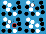
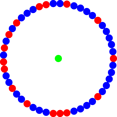
Well-mixed population

This corresponds to the Moran process. An advantageous mutation with r > 1 reaches fixation with a certain probability but this is not guaranteed because of stochastic fluctuations. To visualize the invasion process, individuals are arranged on a circle (see figure to the left) but there is no underlying population structure that defines local neighborhoods.

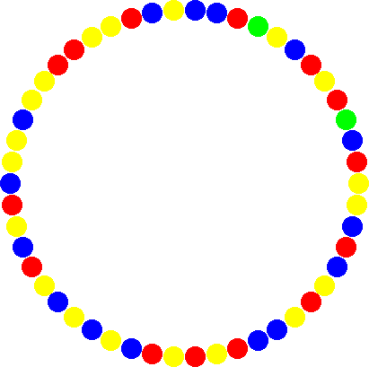
Regular lattices

A mutant invading a resident population with a structure where every individual occupies the site of a square lattice. Here, the offspring replaces a randomly drawn neighbor of the reproducing individual rather than any individual. Consequentially, successful mutants form a cluster that slowly grows (see figure to the left). Interestingly, such symmetrical population structures do not affect the fixation probability of the mutant, i.e. it is the same as in the well-mixed populations. This is an example of an isothermal graph. However, the population structure has significant effects on the average time to fixation. The population structure slows down the spreading speed of the mutants leading to much longer fixation times.

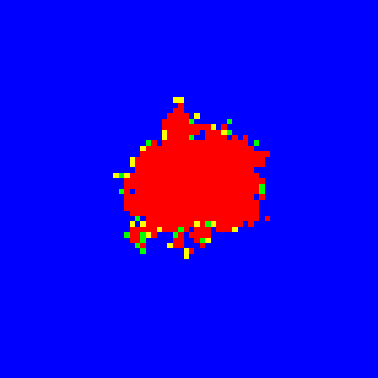
Linear chains

The simplest and most intuitive example of an evolutionary suppressor is the linear chain, where each reproducing individual replaces the neighbor to the right. In this case residents and mutants will co-exist for some time but eventually the mutants are 'washed-out' unless the mutation occurred in the leftmost node (see figure to the left, time runs from top to bottom). This node is never replaced and thus, mutants can reach fixation only if the mutation occurs there. Consequentially, the odds for the mutant to reach fixation are simply 1/N irrespective of the mutant's fitness r - selection is eliminated and random drift rules. Such structural arrangements are important for the somatic evolution of cancer and can be found for example in epithelial tissue where the leftmost node would correspond to a stemm cell.

Stars

The simplest example of an evolutionary amplifier is the star structure where a central hub is connected to all leaf-nodes along the periphery and the peripherial leafs are only connected to the hub. This is no longer an isothermal graph. It is easy to see that the 'temperature', i.e. the sum over the weights of incoming edges, of the hub is much higher than for the peripherial nodes. This structure has the suprising property to amplify selection and suppress random drift. A single mutant with fitness r on a star structure has the same chance to reach fixation as a mutant with fitness r² in a mixed population, i.e. beneficial mutations are more likely to reach fixation on stars. However, nothing is for free and so the increase in fixation probability also leads to an increase of the average fixation time. To illustrate this, the fixation probability of a mutant here is the same as in the well-mixed case but to actually reach fixation it takes much longer on the star (i.e. r_star = sqrt(r_mixed)).

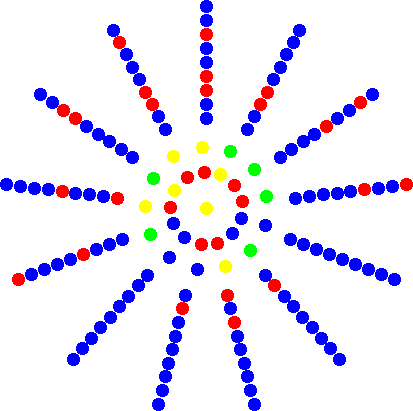Super-stars

Quite amazingly, it is possible to improve evolutionary amplification beyond the star structure. The super-stars are star-like structures but have directed links where the central hub is connected to all nodes arranged in different 'petals'. Each of the nodes in one petal feeds into a chain of nodes that is connected back to the hub. The number of links (i.e. the length of the chain) that separate any two petal-nodes determines the amplification factor K. In the figure to the left an example with K = 4 is shown. On the superstar, a single mutant with fitness r has the same chance to reach fixation as a mutant in a mixed population with fitness r^K. Intriguingly, it is clear that K can be arbitrarily large, which implies that for any mutant with an arbitrarily small fitness advantage, as compared to the resident, fixation can be guaranteed (for N to infinity). The downside is, that in this limit, the average fixation time goes to infinity as well.

Scale-free networks

Scale-free networks are abundant in nature ranging from ecosystems, to gene interaction networks, the world-wide-web and social structures of human society. It turns out that these structures are also weak evolutionary amplifiers but in contrast to the superstars, their structure is very robust. Intuitively it is easily understood why these structures amplify selection: the characteristics of a scale-free network are that it contains few hubs, i.e. nodes with larger numbers of connections but the vast majority has only few connections. This immediately reminds of the hub-leaf structure of stars. Thus, qualitatively it is not so suprising that scale-free graphs enhance selection but quite surprisingly, the actual amplification now depends on the fitness of the mutant. The amplification is almost as good as on stars for only slighlty beneficial mutants but then decreases as the fitness of the mutant increases. Thus, scale-free networks selectively support weakly beneficial mutants.

VirtualLab

Along the bottom of the VirtualLab are several buttons to control the execution and the speed of the simulations. Of particular importance are the Param button and the data views pop-up list on top. The former opens a panel that allows to set and change various parameters concerning the game as well as the population structure, while the latter displays the simulation data in different ways.

Color code:	Resident	Mutant
	New resident	New mutant

Note: The yellow and green strategy colors are very useful to get an intuition of the activitiy in the system.

Java applet on the Moran process. Sorry, but you are missing the fun part!

	Controls
Params	Pop up panel to set various parameters.
Views	Pop up list of different data presentations.
Reset	Reset simulation
Run	Start/resume simulation
Next	Next generation
Pause	Interrupt simulation
Slider	Idle time between updates. On the right your CPU clock determines the update speed while on the left updates are made roughly once per second.
Mouse	Mouse clicks on the graphics panels generally start, resume or stop the simulations.

	Data views
Structure - Strategy	Snapshot of the spatial arrangement of strategies. Mouse clicks cyclically change the strategy/type of the respective site for the preparation of custom initial configurations.
Mean frequency	Time evolution of the strategy frequencies.
Structure - Fitness	Snapshot of the spatial distribution of payoffs.
Mean Fitness	Time evolution of the mean payoff of each strategy together with the average population payoff.
Histogram - Fitness	Histogram of payoffs for each strategy.

Game parameters

The list below describes only the parameters relevant for the Moran process. Follow the link for a complete list and detailed descriptions of all other parameters such as spatial arrangements or update rules on the player and population level.

Resident fitness:: fitness of resident.
Mutant fitness:: fitness of mutant. Only the relative performance of mutants as compared to residents matters.
Init Resident, Init Mutant:: initial fractions of residents and mutants. If they do not add up to 100%, the values will be scaled accordingly. Setting the residents to 100% and mutants to zero puts a single mutant in a resident population.