Data views of VirtualLabs

Strategies in well-mixed populations

In well-mixed or unstructured populations individuals are drawn as colored dots arranged on a circle. The location of the dots has no implications as interactions are equally likely to occur between any members of the population.

The color of each site denotes its strategy. The number of strategies depends on the game presently studied. Intermediate or lighter shades of color indicate sites that have just reassessed and changed their strategy. This is a very useful indicator for the activity in the system.

For larger population sizes, it may not be possible to display this view because the dot size becomes less than a pixel on the screen.

Strategies on a linear chain

Individuals can be arranged on a linear chain and interact with their neighbors on both or just one side. The number of interaction partners is determined by the neighborhood size. Subsequent states of the population are added as a new line to the bottom of the display area such that time runs from top to bottom.

The sample snapshot to the left shows an asymmetric population structure with fixed boundary conditions where individuals interact only with one neighbor to the right.

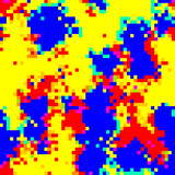Strategies on rectangular lattices

Setting the geometry to square gives a rectangular lattice with different numbers of neighbors. A neighborhood size of four and eight (3×3)gives the von Neumann and Moore neighborhood but larger neighborhoods covering individuals in a 5×5, 7×7 etc. area are also possible.

Note that this view is not accessible for all types of geometries. It can be displayed only population structures corresponding to a regular lattice.

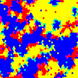Strategies on honeycomb lattices

The hexagonal geometry gives a honeycomb structure where each player has six neighbors.

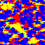Strategies on triangular lattices

The third and last possibility of regular lattices in two dimensions is the triangular lattice where each player has three neighbors.

Strategies on a star structure

In a star-structured population, all nodes (leafs) are connected to a central hub. Thus, the hub has N-1 neighbors but all other individuals have just a single neighbor (the hub), where N denotes the population size.

Strategies on a super-star structure

The super-stars are star-like structures but have directed links where the central hub is connected to all nodes arranged in different 'petals'. Each of the nodes in one petal feeds into a chain of nodes that is connected back to the hub. The number of links (i.e. the length of the chain) that separate any two petal-nodes determines a so-called amplification factor K.

On the left two examples are shown: the top panel shows the links and their direction for a super-star with 5 petals and K=3; the bottom panel shows a super-star with K=4 and 13 petals as it is displayed by the virtuallabs.

Strategies on arbitrary structures

The default representation of the population structure is to draw colored dots arranged in a circle (just as for well-mixed populations) but then to draw the links between interacting individuals. While it may not be possible to identify all connections of one individual it still gives an impression of the connection density and of features of the algorithm used to initialize the population structure.

Mean frequencies of strategies

Mean frequencies of all strategies in the population as a function of time. The line colors distinguish the different strategies and the three horizontal black ;lines indicate the 25%, 50% and 75% levels. The actual time scale along the x-axis is determined by the chosen report frequency.

Strategy frequencies in 2D Phase plane

Mean frequencies of strategies shown in a 2D phase plane. In the case of voluntary participation in public goods games and population dynamics a convenient transformation exists that maps the simplex S₃ presentation onto the 2D phase plane.

The example on the left illustrates a stable limit cycle that is produced by the the feedback mechanism between public goods games and population sizes.

Strategy frequencies on S₃ simplex

Mean frequencies of strategies shown in the simplex S₃. In the case of three strategy types it is convenient to plot the strategies in the simplex S₃ which takes into account that the frequencies of the strategies must sum up to one. In particular this view is useful to investigate cycling or spiraling dynamics.

Strategy frequencies on S₄ simplex - invariant manifold

In some cases such as the reward & punishment scenarios the simplex S₄ is foliated by invariant manifolds W_k. This means that the state of the system always remains on one particular manifold. Strictly speaking this is true only for infinite population sizes. This manifold is determined by x₁ x₃/(x₂ x₄) = k being constant. Since k will change over time in any finite population, the current value of k is shown below the manifold.

The picture shows sample trajectories for punishment & reputation in pairwise interactions.

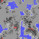Payoffs in structured populations

The gray shade of each site indicates the payoff achieved. White sites have achieved the maximum payoff and black ones the minimum. In addition, sites earning payoffs of a homogenous population of a particular strategy are colored in light shades of that strategies' color. For example, on the square lattice depicted to the left, pale blue indicates sites that obtain payoffs of mutual cooperation and the pale red ones of mutual defection.

Just as for the strategies above, the different population structures are shown whenever possible. This ranges from well-mixed populations and different kinds of lattices to more general structures such as random regular graphs or scale-free networks.

Mean Fitness

Mean fitness for each strategy type as well as the average population fitness. The fitness of the different strategies are indicated with different colors and the average population payoff is shown in black. The y-axis runs from the minimum to the maximum payoff and the pale blue and pale red horizontal lines indicate the payoffs for mutual cooperation and mutual defection, respectively. Note that this means the population payoff always remains within these limits. As before, the actual time scale along the x-axis is determined by the chosen report frequency.

Payoff histograms

Histogram of the payoffs for each strategy type. The different strategies are indicated by different colors and the name of the strategy is given in the top left corner of the respective panel. To improve the readability of the histograms, the ordinate is automatically rescaled. The current scale is specified in the top left corner of each panel. For example, a current scale of 25% means that the maximum for this panel is scaled to 25%. In the defector panel the payoff for mutual defection is marked by pale red lines straddling the corresponding bin in the histogram. Similarly, in the cooperator panel the payoff for mutual cooperation is marked by pale blue lines.

Continuous strategies on rectangular lattices

The shade of grey of each site denotes its strategy, e.g. the amount of the cooperative investment. Dark shades refer to low and light shades to high investors.

Setting the geometry to square gives a rectangular lattice with either four or eight neighbors, i.e. von Neumann or Moore neighborhood. In addition the geometry can be hexagonal or triangular as before.

Note that this view is not accessible for all types of geometries. It can be displayed only population structures corresponding to a regular lattice.

Payoffs on rectangular lattices

The gray shade of each site indicates the payoff achieved. White sites achieve the maximum and black sites the minimum payoff.

Average strategy

In analogy to the mean frequency of the different strategies in the discrete scenario this displays the mean strategy, e.g. the mean propensity to cooperate or the mean investment level as a solid black line. The pale blue and red lines indicate the maximum and minimum investments - to give a rough idea of the variance in the population.

Note that the range of strategies may not be bounded. In that case the range is simply chosen large enough - e.g. twice the optimum investment level.

Strategy distribution

In order to get a better idea of the strategy composition of the population a histogram of the strategy frequencies is available. The range of possible strategies is divided into 100 bins.

The sample image on the left shows the strategy distribution shortly after evolutionary branching. The population spontaneously splits into two distinct phenotypic clusters. More on continuous games and evolutionary branching can be found in the tutorial on the Evolutionary Origin of Cooperators and Defectors.

Strategy density distribution

The density distribution of the strategies is shown as a function of time. The ordinate denotes the trait interval and the abscissa the time axis. The shades of grey indicate the density (frequency) of a particular trait in the population ranging from white (none) to black (1/3), red (2/3) and finally yellow (all). Generally the shades are grey such as in the example to the left depicting the branching process in the Evolutionary Origin of Cooperators and Defectors.

Payoff levels

This view displays the mean population payoff (black) together with the minimum (pale red) and maximum (pale blue) payoffs for one player.

Note that the accessible payoffs may not be bounded. In that case the maximum value is chosen to be sufficiently large e.g. the payoff for strategies investing twice the optimum.

Payoff distribution

In order to get a better idea of the distribution in the population, a histogram of the strategy payoffs is available. The range of possible payoffs is divided into 100 bins.